


Load balancing algorithm selection determines the method and prioritization for distributing connections or HTTP requests across available servers.
The load balancing algorithm is changed using NSX Advanced Load Balancer UI and NSX Advanced Load Balancer CLI. Select a local server load-balancing algorithm using the Load Balance Algorithm field in General tab under Pools screen. Changing a pool’s LB algorithm will only affect new connections or requests, and will have no impact on existing connections. The available options are:
Consistent Hash
Core Affinity
Fastest Response
Fewest Servers
Least Connections
Least Load
Round Robin
Topology
Consistent Hash
New connections are distributed across the servers using a hash that is based on a key specified in the field that appears below the Load Balance Algorithm field or in a custom string provided by the user through the avi.pool.chash DataScript function. Below is an example of persisting on a URI query value:
hash = avi.http.get_query("r")
if hash then
avi.pool.select("Pool-Name")
avi.pool.chash(hash)
end
This algorithm inherently combines load balancing and persistence, which minimizes the need to add a persistence method. This algorithm is best for load balancing large numbers of cache servers with dynamic content. It is ‘consistent’ because adding or removing a server does not cause a complete recalculation of the hash table. For the example of cache servers, it will not force all caches to have to re-cache all content. If a pool has nine servers, adding a tenth server will cause the pre-existing servers to send approximately 1/9 of their hits to the newly-added server based on the outcome of the hash. Hence, persistence may still be valuable. The rest of the server’s connections will not be disrupted. The available hash keys are:
Field |
Description |
|---|---|
Call-ID |
Specifies the Call ID field in the SIP header. With this option, SIP transactions with new call IDs are load balanced using consistent hash, while existing call IDs are retained on the previously chosen servers. The state of existing call IDs is maintained for an idle timeout period defined by the ‘Transaction timeout’ parameter in the Application Profile. The state of existing call IDs is relevant for the underlying TCP/ UDP transport state for the SIP transaction remains the same. |
Custom Header |
Specify the HTTP header to use in the Custom Header field, such as Referer. This field is case-sensitive. If the field is blank or if the header does not exist, the connection or request is considered a miss and will hash to a server. |
Custom String |
Consistent Hash based on a custom string. |
Source IP Address |
Source IP Address of the client. |
Source IP Address and Port |
Source IP Address and Port of the client. |
HTTP URI |
It includes the host header and the path. For instance, www.avinetworks.com/index.htm. |
The custom string Consistent Hash algorithm can be used in pools which are members of pool group also.
The same server is selected only if the same pool is selected by pool group. If a different pool is selected by the pool group, the traffic is load balanced to a server in a newly selected pool depending on the load balancing algorithm of the corresponding pool.
Core Affinity
Each CPU core uses a subset of servers, and each server is used by a subset of cores. Essentially it provides a many-to-many mapping between servers and cores. The sizes of these subsets are parameterized by the variable lb_algorithm_core_nonaffinity in the pool object. When increased, the mapping increases up to the point where all servers are used on all cores.
If all servers that map to a core are unavailable, the core uses servers that map to the next (with wraparound) core.
Fastest Response
New connections are sent to the server that is currently providing the fastest response to new connections or requests. This is measured as time to the first byte. In the End-to-End Timing chart, this is reflected as Server RTT plus App Response time. This option is best when the pool’s servers contain varying capabilities or they are processing short-lived connections. A server that is having issues, such as a lost connection to the datastore containing images, will generally respond very quickly with HTTP 404 errors. It is best practice when using the fastest response algorithm to also enable the Passive Health Monitor, which recognizes and adjusts for scenarios like this by taking into account the quality of server response, not just speed of response.
A server that is having issues, such as a lost connection to the datastore containing images, will generally respond very quickly with HTTP 404 errors. Use the Fastest Response algorithm with the Passive Health Monitor, which recognizes and adjusts for scenarios like this.
Fewest Servers
Instead of attempting to distribute all connections or requests across all servers, NSX Advanced Load Balancer will determine the fewest number of servers required to satisfy the current client load. Excess servers will no longer receive traffic and may be either de-provisioned or temporarily powered down. This algorithm monitors server capacity by adjusting the load and monitoring the server’s corresponding changes in response latency. Connections are sent to the first server in the pool until it is deemed at capacity, with the next new connections sent to the next available server down the line. This algorithm is best for hosted environments where virtual machines incur a cost.
Least Connections
New connections are sent to the server that currently has the least number of outstanding concurrent connections. This is the default algorithm when creating a new pool and is best for general-purpose servers and protocols. New servers with zero connections are introduced gracefully over a short period of time through the Connection Ramp setting in the . This feature slowly brings the new server up to the connection levels of other servers within the pool.
NSX Advanced Load Balancer uses Least Connections as the default algorithm because generally provides an equal distribution when all servers are healthy, and yet is adaptive to slower or unhealthy servers. It works well for both long-lived and quick connections.
A server that is having issues, such as rejecting all new connections, may have a concurrent connection count of zero and be the most eligible to receive all new connections. NSX Advanced Load Balancer recommends using the Least Connections algorithm with the Passive Health Monitor which recognizes and adjusts for scenarios like this. A passive monitor will reduce the percent of new connections sent to a server based on the responses it returns to clients.
In the application profile, connections are not managed by the flowtable when System-syslog is selected. It is because syslog only communicates in one direction and does not maintain a steady connection with the server. As a result, the Least Connection algorithm is not applicable to System-syslog.
Least Load
New connections are sent to the server with the lightest load, regardless of the number of connections that the server has. For example, if an HTTP request requiring a 200-kB response is sent to a server and a second request that will generate a 1-kB response is sent to a server, this algorithm will estimate that —based on previous requests— the server sending the 1-kB response is more available than the one still streaming 200 kB. The idea is to ensure that a small and fast request does not get queued behind a very long request. This algorithm is HTTP-specific. For non-HTTP traffic, the algorithm will default to the least connections algorithm.
Round Robin
New connections are sent to the next eligible server in the pool in sequential order. This static algorithm is best for basic load testing but is not ideal for production traffic because it does not take the varying speeds or periodic hiccups of individual servers into account. A slow server will still receive as many connections as a better-performing server.
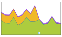
In the example illustration, a server was causing significant app response time in the end-to-end timing graph as seen by the orange in the graph. By switching from the static round-robin algorithm to a dynamic LB algorithm (the blue config event icon at the bottom), NSX Advanced Load Balancer successfully directed connections to servers that were responding to clients faster, virtually eliminating the app response latency.
Fewest Tasks
Load is adaptively balanced, based on server feedback. This algorithm is facilitated by an External Health Monitor and is configurable through the NSX Advanced Load Balancer CLI and REST API. The Fewest Tasks algorithm is not configurable from the NSX Advanced Load Balancer UI.
Configuring Using NSX Advanced Load Balancer CLI
configure pool foo
lb_algorithm lb_algorithm_fewest_tasks
save
An external health monitor can feedback a number (for example, 1-100) to the algorithm by writing data into the <hm_name>.<pool_name>.<ip>.<port>.tasks file. Each output from this file will be used as feedback to the algorithm. The range of numbers provided as feedback and the send interval of the health monitor can be adjusted to tune the load balancing algorithm behavior to the specific environment.
For example, consider a pool p1 with 2 back-end servers, s1 and s2. Assume that the health monitor ticks every 10 seconds (send-interval), and sends back feedback of 100 (high load) and 10 (low load). At time t1, s1 and s2 are set with 100 tasks and 10 tasks respectively. Now, if you send 200 requests, the first 90 would go to s2, since it had 90 more units available. The next 110 would be sent equally to s1 and s2. At time t2 = t1 + 10 sec, s1 and s2 get replenished to the new data provided by the external health monitor.
The following is an example script for use by the external health monitor:
#!/usr/bin/python
import sys
import httplib
import os
conn = httplib.HTTPConnection(sys.argv[1]+':'+sys.argv[2])
conn.request("GET", "/")
r1 = conn.getresponse()
print r1
if r1.status == 200:
print r1.status, r1.reason ## Any output on the screen indicates SUCCESS for health monitor

try:
fname = sys.argv[0] + '.' + os.environ['POOL'] + '.' + sys.argv[1] + '.' + sys.argv[2] + '.tasks'
f = open(fname, "w")
try:
f.write('230') # Write a string to a file - instead of 230 - find the data from the curl output and feed it.
finally:
f.close()
except IOError:
pass
You can use the show pool <foo> detail and show pool <foo> server detail commands to see detailed information about the number of connections being sent to the servers in the pool.
Weighted Ratio
NSX Advanced Load Balancer does not include a dedicated weighted ratio algorithm. Instead, weight may be achieved through the ratio, which may be applied to any server within a pool. The ratio may also be used with any load balancing algorithm. With the ratio setting, each server receives statically adjusted ratios of traffic. If one server has a ratio of 1 (the default) and another server has a ratio of 4, the server set to 4 will receive 4 times the amount of connections it otherwise would. For instance, using the least connections, one server may have 100 concurrent connections while the second server has 400.
