


Capacity analytics helps you assess the utilization and capacity remaining in objects across your environment. An evaluation of the historical utilization of resources generates a projection of the future workload. You can plan for infrastructure procurement or migrations based on the projection and avoid the risk of capacity shortage and high infrastructure costs.
Capacity analytics uses the capacity engine to assess historical trends, which include utilization peaks. The engine chooses an appropriate projection model to predict the future workload. The amount of historical data that is considered depends on the amount of historical utilization data.
Capacity Engine and Calculations
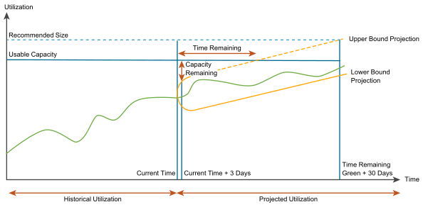
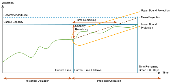
The capacity engine analyzes historical utilization and projects future workload by using real-time predictive capacity analytics, which is based on an industry-standard statistical analysis model of demand behavior. The engine takes the Demand and Usable Capacity metrics as input and generates the output metrics, which are Time Remaining, Capacity Remaining, Recommended Size, and Recommended Total Capacity, as shown in the following figure.

The projection window for the capacity engine is 1 year into the future. The engine consumes data points every 5 minutes to ensure real-time calculation of output metrics.
The capacity engine projects the future workload in a projected utilization range. The range includes an upper bound projection and a lower bound projection. Capacity calculations are based on the time remaining and risk level. The engine considers the upper bound projection for a conservative risk level and the mean of the upper bound projection and lower bound projection for an aggressive risk level. For more information about setting risk levels, see, Capacity Details in the Configuring Policies chapter of the VMware vRealize Operations Configuration Guide.
The capacity engine calculates the time remaining, capacity remaining, recommended size, and recommended total capacity.
- Time Remaining
- The number of days remaining till the projected utilization crosses the threshold for the usable capacity. The usable capacity is the total capacity excluding the HA settings.
- Capacity Remaining
- The largest difference between the usable capacity and the projected utilization between now and 3 days into the future. If the projected utilization is above 100% of the usable capacity, the capacity remaining is 0.
- Recommended Size
-
The maximum projected utilization for the projection period from the current time to 30 days after the warning threshold value for time remaining. The warning threshold is the period during which the time remaining is green. The recommended size excludes HA settings.
If the warning threshold value for time remaining is 120 days, which is the default value, the recommended size is the maximum projected utilization 150 days into the future.
vRealize Operations caps the recommended size that is generated by the capacity engine to keep the recommendations conservative.- vRealize Operations caps an oversized recommended size at 50% of the currently allocated resources.
For example, a virtual machine that is configured with 8 vCPUs has never used more than 10% CPU historically. Instead of recommending a reclaim of 7 vCPUs, the recommendation is capped to reclaiming 4 vCPUs.
- vRealize Operations caps an undersized recommended size at 100% of the currently allocated resources.
For example, a virtual machine that is configured with 4 vCPUs has been constantly running very hot historically. Instead of recommending the addition of 8 vCPUs, the recommendation is capped at adding 4 vCPUs.
- vRealize Operations caps an oversized recommended size at 50% of the currently allocated resources.
- Recommended Total Capacity
-
The maximum projected utilization for the projection period from the current time to 30 days after the warning threshold value for time remaining. The recommended total capacity includes HA settings.
For example, if the warning threshold value for time remaining is 120 days, which is the default value, the recommended size is the maximum projected utilization including HA values, 150 days into the future.
Note: Recommended total capacity is not available for objects.
The following figure shows the capacity calculations for a conservative risk level.
The following figure shows the capacity calculations for an aggressive risk level.
- If HA is not enabled in VC then Usable Capacity = Total Capacity. In this case, the Usable Capacity value can be 0 only if there are no hosts in the Cluster.
- If HA is enabled, then Usable Capacity can be 0 in the following cases:
- There are no hosts in the cluster.
- HA is configured incorrectly. For example: it can be configured to 100% percent. Please check the HA configuration in vCenter.
- HA Active host count is less than 2.
- The host is not HA Active if:
- Host is in Maintenance Mode.
- Host is Powered Off.
- Value of “runtime.dasHostState” property is not equal to “connectedToMaster” or “master”. This can be because of some network issues between the hosts.
Utilization Peaks
The historical utilization of resources can have peaks, which are periods of maximum utilization. The projection of future workload depends on the types of peaks. According to the frequency of peaks, they can be momentary, sustained, or periodic.
- Momentary Peaks
- Short-lived peaks that are a one-time occurrence. The peaks are not significant enough to require additional capacity, so they do not impact capacity planning and projection.
- Sustained Peaks
- Peaks that last for a longer time and impact projections. If a sustained peak is not periodic, the impact on the projection lessens over time because of exponential decay.
- Periodic Peaks
- Peaks that exhibit cyclical patterns or waves. The peaks can be hourly, daily, weekly, monthly, during the last day of the month, and so on. The capacity engine also detects multiple overlapping cyclical patterns.
Projection Models
The capacity engine uses projection models to generate projections. The engine constantly modifies projections and chooses the model that best fits the pattern of historical data. The projection range predicts the general usage pattern that covers 90% of the future data points. Projection models can be linear or periodic.
- Linear Models
-
Models that have a steadily increasing or decreasing trend. Multiple linear models run in parallel and the capacity engine chooses the best model.
Examples of linear models are linear regression and autoregressive moving average (ARMA).
- Periodic Models
-
Models that discover periodicity of various lengths, such as hours, days, weeks, months, or the last day of the week or month. Periodic models detect square waves that represent batch jobs and handle data streams that contain multiple overlapping periodic patterns. These models ignore random noise.
Examples of periodic models are fast Fourier transforms (FFTs), pulses (edge detection), and wavelets.
Forecast In Trend Views
Forecasts are generated based on the time range specified in the view settings and are forecasted for the number of days specified in the forecast setting. The forecast is generated based on 3 main algorithms. Change-point detection to find sections of the history with significant changes, linear regression to find linear trends, and cyclical analysis to identify periodic patterns.
Historical Data Window
The capacity engine captures historical data over a period of time depending on the historical data window. The historical data window that the engine uses is an exponential decay window.
The exponential decay window is a window of unlimited size in which the capacity engine gives more importance to the most recent data points. Beginning from the projection calculation start point, the engine consumes all the historical data points and weighs them exponentially, based on how far back in time they are.
